Designing Machine Learning Pipelines Using Reinforcement Learning

Preface
When developing a model, data scientists work in some development environment tailored for Statistics and Machine Learning (Python, R etc) and are able to train and test models all in one 'sandboxed' environment while writing relatively little code. This is great for building interactive prototypes with fast time to market — they are not productionised, low latency systems though!
This is the 2nd in a series of articles, namely ' Being a Data Scientist does not make you a Software Engineer! ' which covers how you can architect an end-to-end scalable Machine Learning (ML) pipeline.
Revision
Hopeful l y you have gone through the 1st part of the series, where we introduced the basic architectural styles, design patterns and the SOLID principles.

📌 TL;DR: In case you haven't read it, let's repeat the 'holy grail' — i.e. the problem statement that a production-ready ML system should try to address:
The main objectives are to build a system that:
▸ Reduces latency;
▸ Is integrated but loosely coupled with the other parts of the system, e.g. data stores, reporting, graphical user interface;
▸ Can scale both horizontally and vertically;
▸ Is message driven i.e. the system communicates via asynchronous, non-blocking message passing;
▸ Provides efficient computation with regards to workload management;
▸ Is fault-tolerant and self healing i.e. breakdown management;
▸ Supports batch and real-time processing.

🎦 Scene Setting: So by now you have seen the fundamental concepts of Software Engineering and you already are a seasoned Data Scientist.
Without further ado, let's put two and two together…
For each of the ML Pipeline steps I will be demonstrating how to design a production-grade architecture. I will intentionally not be referring to any specific technologies (apart from a couple of times that I give some examples for demonstration purposes).
✏️ N.B.: If you need to refresh on the ML pipeline steps, take a look at this resource.
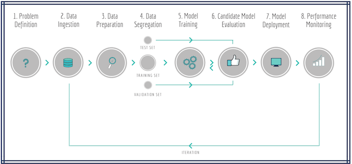
Architecting a ML Pipeline
Traditionally, pipelines involve overnight batch processing, i.e. collecting data, sending it through an enterprise message bus and processing it to provide pre-calculated results and guidance for next day's operations. Whilst this works in some industries, it is really insufficient in others, and especially when it comes to ML applications.
The following diagram shows a ML pipeline applied to a real-time business problem where features and predictions are time sensitive (e.g. Netflix's recommendation engines, Uber's arrival time estimation, LinkedIn's connections suggestions, Airbnb's search engines etc).

It comprises of two clearly defined components:
- Online Model Analytics: The top row represents the operational component of the application i.e. where the model is applied for real-time decision making.
- Offline Data Discovery: The bottom row represents the learning component i.e. analysis on historical data to create the ML model in a batch-processing mode.
We will now take this simplified diagram and unfold its inner workings.
— ①: Data Ingestion
Data collection.
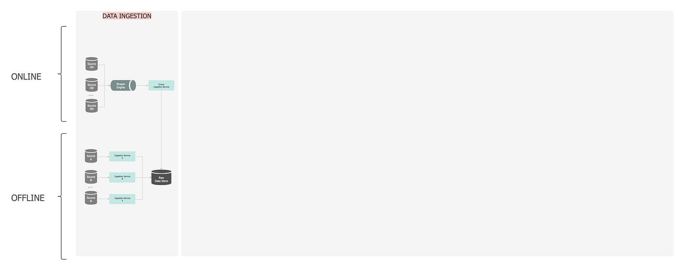
Funnelling incoming data into a data store is the first step of any ML workflow. The key point is that data is persisted without undertaking any transformation at all, to allow us to have an immutable record of the original dataset. Data can be fed from various data sources; either obtained by request (pub/sub) or streamed from other services.
NoSQL document databases are ideal for storing large volumes of rapidly changing structured and/or unstructured data, since they are schema-less. They also offer a distributed, scalable, replicated data storage.
Offline
In the offline layer, data flows into the Raw Data Store via an Ingestion Service — a composite orchestration service, which encapsulates the data sourcing and persistence. Internally, a repository pattern is employed to interact with a data service, which in return interacts with the data store. When the data is saved in the database, a unique batch-id is assigned to the dataset, to allow for efficient querying and end-to-end data lineage and traceability.
To be performant, the ingestion distribution is twofold:
• there is a dedicated pipeline for each dataset so all of them are processed independently and concurrently, and
• within each pipeline, the data is partitioned to take advantage of the multiple server cores, processors or even servers.
Spreading the data preparation across multiple pipelines, horizontally and vertically, reduces the overall time to complete the job.
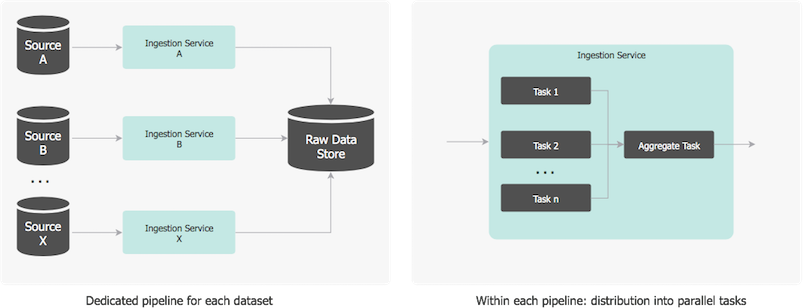
The ingestion service runs regularly on a schedule (once or multiple times per day) or on a trigger: a topic decouples producers (i.e. the sources of data) from consumers (in our case the ingestion pipeline), so when source data is available, the producer system publishes a message to the broker, and the embedded notification service responds to the subscription by triggering the ingestion. The notification service also broadcasts to the broker that the source data has been successfully processed and is saved in the database.
Online
In the online layer, the Online Ingestion Service is the entry point to the streaming architecture as it decouples and manages the flow of information from data sources to the processing and storage components, by providing reliable, high throughput, low latency capabilities. It functions as an enterprise-scale 'Data Bus'. Data is saved in a long term Raw Data Store, but is also a pass-through layer to the next online streaming service, for further real-time processing.
Example technologies used here can be Apache Kafka (pub/sub messaging system) and Apache Flume (data collection to long term db), but there are more you will come across, depending on your enterprise's tech stack.
— ②: Data Preparation
Data exploration, data transformation and feature engineering.
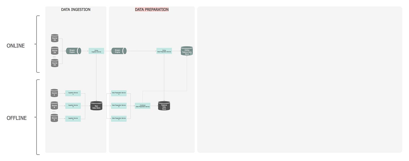
Once the data is ingested, a distributed pipeline is generated which assesses the condition of the data, i.e. looks for format differences, outliers, trends, incorrect, missing, or skewed data and rectify any anomalies along the way. This step also includes the feature engineering process. There are three main phases in a feature pipeline: extraction, transformation and selection.

As this is the most complex part of a ML project, introducing the right design patterns is crucial, so in terms of code organisation having a factory method to generate the features based on some common abstract feature behaviour as well as a strategy pattern to allow the selection of the right features at run time is a sensible approach. Both feature extractors and transformers should structured with composition and re-usability in mind.
Selecting the features can be left to the caller, or can be automated e.g. apply a chi-squared statistical test to rank the impact of each feature on the concept label and discard the less impactful features prior to model training. A series of selector APIs can be defined to enable this. Either way, to ensure consistency on the features used as model inputs and at scoring, a unique id is assigned to each feature set.
Broadly speaking, a data preparation pipeline should be assembled into a series of immutable transformations, that can easily be combined. This is where the significance of testing and high code coverage becomes an important factor for the project's success.
Offline
In the offline layer, the Data Preparation Service, is triggered by the completion of the ingestion service. It sources the Raw Data, undertakes all the feature engineering logic, and saves the generated features in the Feature Data Store.
The same partitioning applies here too (i.e. dedicated pipelines / parallelism).
Optionally, the features from multiple data sources can be combined, so a 'join/sync' task is designed to aggregate all the intermediate completion events and create these new, combined features. In the end, the notification service broadcasts to the broker this process is complete and the features are available.
When each data preparation pipeline finishes, the features are also replicated to the Online Feature Data Store, so that the features can be queried with low latency for real-time prediction.
Online
The raw data is streamed from the ingestion pipeline into the Online Data Preparation Service. The generated features are stored in an in-memory Online Feature Data Store where they can be read at low latency at prediction time, but are also persisted in the long term Feature Data Store for future training. Additionally the in-memory database can be pre-warmed by loading features from the long term Feature Data Store.
Continuing the earlier tech stack example, a frequently used streaming engine is Apache Spark.

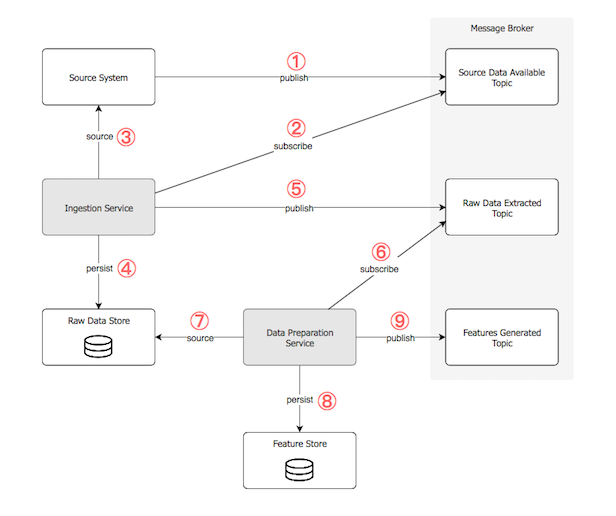
🔍 Offline Drill Through: If we were to drill through the offline Ingestion and the Data Preparation services interaction, we would have something like below:
• (1) One or more data producers publish events to a designated 'Source Data Available' topic of the message broker, that the data is ready for consumption.
• (2) The Ingestion Service is listening to the topic.
• Once the respective event is received, it handles it by: (3) sourcing the data and (4) persisting it in its raw format in the data store.
• (5) When the process finishes, it raises a new event to the 'Raw Data Extracted' topic to notify that the raw data is ready.
• (6) The Data Preparation Service is listening to the topic.
• Once the respective event is received, it handles it by: (7) sourcing the raw data, preparing it and engineering new features and (8) persisting the features in the data store.
• (9) When the process finishes, it raises a new event to the 'Features Generated' topic to notify that the features have been generated.
— ③: Data Segregation
Split subsets of data to train the model and further validate how it performs against new data.
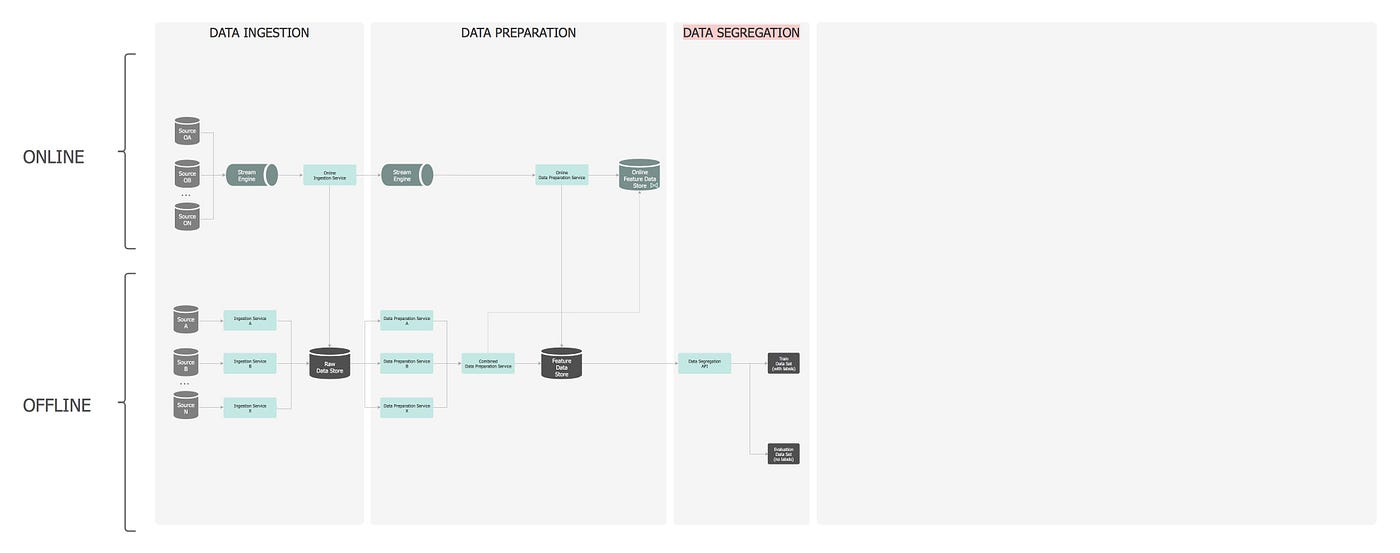
The fundamental goal of the ML system is to use an accurate model based on the quality of its pattern prediction for data that it has not been trained on. As such, existing labelled data is used as a proxy for future/unseen data, by splitting it into training and evaluation subsets.
There are many strategies to do that, four of the most common ones are:
• Use a default or custom ratio to split it into the two subsets, sequentially i.e. in the order it appears in the source, making sure there is no overlapping. For instance use the first 70% of data for training and the subsequent 30% of data for testing.
• Use a default or custom ratio to split it into the two subsets via a random seed. For instance select a random 70% of the source data for training and the complement of this random subset for testing.
• Use either of the methods above (sequential vs. random) but also shuffle the records within each dataset.
• Use a custom injected strategy to split the data, when an explicit control over the separation is needed.
The data segregation is not a separate ML pipeline as such, but an API or service must be available to facilitate this task. The next two pipelines (model training and evaluation) must be able to call this API to get back the requested datasets. In terms of code organisation, a strategy pattern is necessary so the caller service can select the right algorithm at run time, and obviously the ability to inject the ratio or random seed is needed. Additionally, the API must be able to return the data with or without labels/traits — for training and evaluation respectively.
To protect the caller from specifying parameters that cause an uneven data distribution, a warning should be raised and returned along with the dataset.
— ④: Model Training
Use the training subset of data to let the ML algorithm recognise the patterns in it.
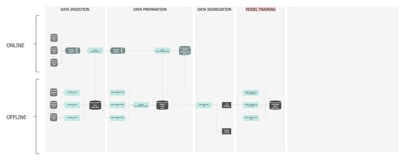
The model training pipeline is offline only and its schedule varies depending on the criticality of the application, from every couple of hours to once a day. Apart from schedulers, the service is also time and event triggered.
It consists of a library of training model algorithms (linear regression, ARIMA, k-means, decision trees etc), which is built in a SOLID way to make provision for continuous development of new model types as well as making them interchangeable. Also containment, using the facade pattern, is a crucial technique for integrating third-party APIs (this is where your Python Jupyter notebook can be wrapped and called too).
There are a few options for parallelisation:
• The simplest form is to have a dedicated pipeline for each model, i.e. all models run concurrently.
• Another idea is to parallelise the training data i.e. the data is partitioned and each partition has a replica of the model. This is preferred for those models that they need all fields of an instance to perform the computation (e.g. LDA, MF).
• A third option is to parallelise the model itself i.e. the model is partitioned and each partition is responsible for the updates of a portion of parameters. It is ideal for Linear models, such as LR, SVM.
• Finally, a hybrid approach can be used, combining one or more options. (For more info I recommend you read this publication).
Model training must be implemented with error tolerance in mind and also data checkpoints and failover on training partitions should be enabled — e.g. each partition can be retrained if the previous attempt fails due to some transient issue (e.g. timeout).

Since we covered the capabilities of this pipeline, let's unpack the workflow: The Model Training Service gets the training configuration parameters (e.g. model type, hyper-parameters, features to be used etc) from the Configuration Service and will then request the training dataset from the Data Segregation API. This dataset is sent to all the models in parallel and once complete, the models, the original configuration, the learned parameters, plus metadata on the training set and timings, will be saved in the Model Candidate Data Store.
— ⑤: Candidate Model Evaluation
Assess the performance of the model using the test subset of data to understand how accurate the prediction is.
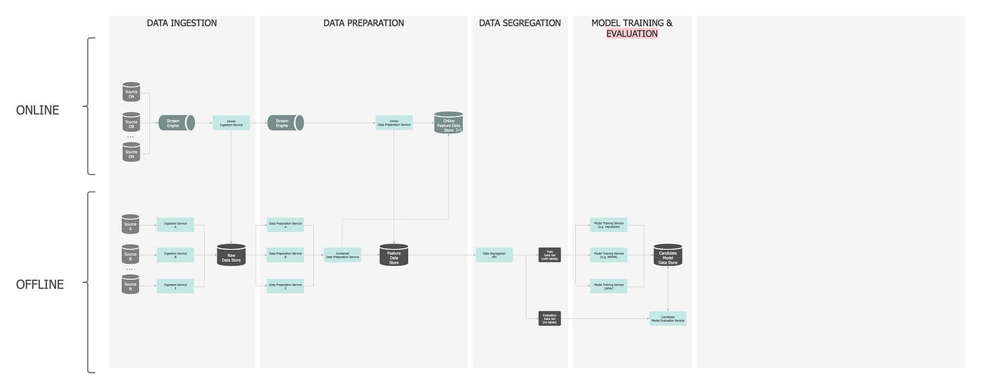
This pipeline is also offline. The predictive performance of a model is evaluated by comparing predictions on the evaluation dataset with true values using a variety of metrics. The "best" model on the evaluation subset is selected to make predictions on future/new instances. A library of several evaluators is designed to provide a model's accuracy metrics (e.g. ROC curve, PR curve), which are also saved against the model in the data store. Again, same patterns are applicable here to allow flexibility on combining and switching between evaluators.

In terms of orchestration, the Model Evaluation Service requests the evaluation dataset from the Data Segregation API, and for each model sourced from the Model Candidate repository, it applies the relevant evaluators. The evaluation results are saved back to the repository. This is an iterative process and hyperparameter optimisation as well as regularisation techniques are also applied to come up with the final model. The best model is marked for deployment. Finally, the notification service broadcasts that a model is ready for deployment.
This pipeline also needs to live up to all the reactive traits.
— ⑥: Model Deployment
Once the chosen model is produced, it is typically deployed and embedded in decision-making frameworks.
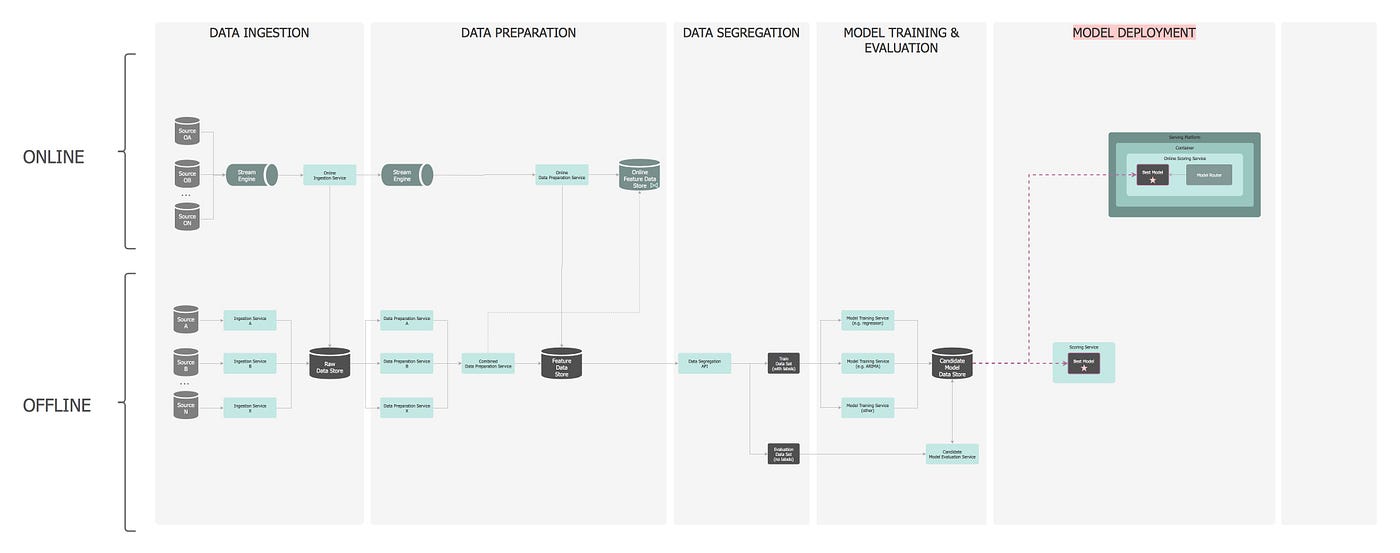
Model deployment is not the end; it is just the beginning!
The best model selected is deployed for offline (asynchronous) and online (synchronous) predictions. More than one models can be deployed at any time to enable safe transition between old and new models — i.e. when
deploying a new model, the services need to keep serving prediction requests.
Traditionally, a challenge in deployment has been that the programming languages needed to operationalise models have been different from those that have been used to develop them. Porting a Python or R model into a production language like C++, C# or Java is challenging, and often results in reduced performance (speed & accuracy) of the original model. There are a few ways to address this issue. In no particular order:
• Rewrite the code in the new language [i.e. translate from Python to CSharp]
• Create custom DSL (Domain Specific Language) to describe the model
• Microservice (accessed through a RESTful API)
• API-first approach
• Containerisation
• Serialise the model and load into a in-memory key-value store
More specifically:
Offline
• In an offline mode, the prediction model can be deployed to a container and run as a microservice to create predictions on demand or on a periodic schedule.
• A different choice is to create a wrapper around it so you gain control over the functions available. Once a batch prediction request is made, you can load it dynamically into memory as a separate process, call the prediction functions, unload it from memory and free up the resources (native handles).
• Finally another approach is to wrap the library into an API and let the caller invoke it directly or wrap it around their service to fully take over the reins of the prediction instrumentation.
In terms of scalability, multiple parallel pipelines can be created to accommodate the load. This involves inconsiderable effort, as the ML models are stateless.
Online
• Here the prediction model can be deployed in a container to a service cluster, generally distributed in many servers behind a queue for load balancing to assure scalability, low latency and high throughput. The clients can send prediction requests as network remote procedure calls (RPC).
• Alternatively, key-value stores (e.g Redis) support the storage of a model and its parameters, which gives a big boost on performance.

✳️ With regards to the actual model deployment activity, it can be automated via a continuous delivery implementation: The required files are packaged, the model is validated by a reliable testing suite and is finally deployed into a running container.
The tests are executed by an automated build pipeline: Short, self-contained, stateless unit tests are evaluated first. If they pass, the prediction model quality is measured in bigger integration or regression tests. When both levels of testing have passed, the application is deployed to the serving environment.
Enabling one-click deployment is ideal.
— ⑦: Model Scoring
Process of applying a ML model to a new dataset in order to uncover practical insights that will help solve a business problem. A.k.a. Model Serving.
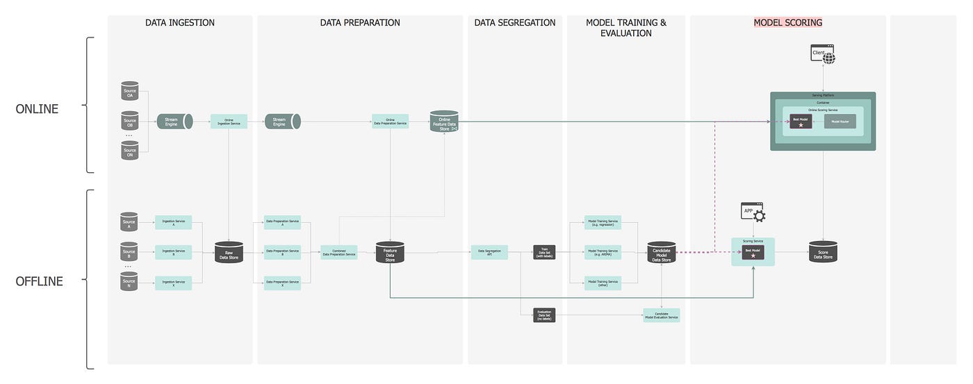
✏️ Model Scoring and Model Serving are two terms that are used interchangeably in the industry. What scoring really means, occurred to me after reading this resource, so before moving on, let's quickly cover the basics, in case this is not clear to you either:
Model Scoring is the process of generating new values, given a model and some new input. The generic term score is used, rather than prediction, as it may result in different types of values:
• A list of recommended items
• Numeric values, for time series models and regression models
• A probability value, indicating the likelihood that a new input belongs to some existing category
• The name of a category or cluster to which a new item is most similar
• A predicted class or outcome, for classification models.

Moving on… Once models are deployed they are used for scoring based on the feature data loaded by previous pipelines or directly from a client service. Models should behave the same in both offline and online modes when serving predictions.
Offline
In the offline layer, the Scoring Service is optimised for high throughput, fire-and-forget predictions for a large collection of data. An application can send an asynchronous request to kick off the scoring process, but needs to wait until the batch scoring process completes before it can access the prediction results. The service prepares the data, generates the features, but also fetches extra features from the Feature Data Store. Once scoring takes place, the results are saved in the Score Data Store. A message is sent to the broker to notify that the scoring has completed. The application is listening to this event and when notified it fetches the scores.
Online
A client sends a request to the Online Scoring Service. It can optionally specify the version of the model to be invoked, so the Model Router inspects the request and sends it to the respective model. Based on the request, similarly to the offline layer, the service prepares the data, generates the features, and optionally fetches extra features from the Feature Data Store. Once scoring takes place, the results are saved in the Score Data Store and then sent back to the client over the network.
Depending on the use-case, scores can also be delivered to the client asynchronously i.e. independently of the request:
• Push: Once the scores are generated, they are pushed to the caller as a notification.
• Poll: Once the scores are generated, they are stored in a low read-latency database; the caller periodically polls the database for available predictions.
In order to minimise the time the system takes to serve the scoring when it receives the request, two methods are employed:
• the input features are stored in a low-read latency in-memory data store,
• predictions precomputed in an offline batch-scoring job are cached for easy access [this is depending on the use-case, as offline predictions might not be relevant].
— ⑧: Performance Monitoring
The model is continuously monitored to observe how it behaved in the real world and calibrated accordingly.
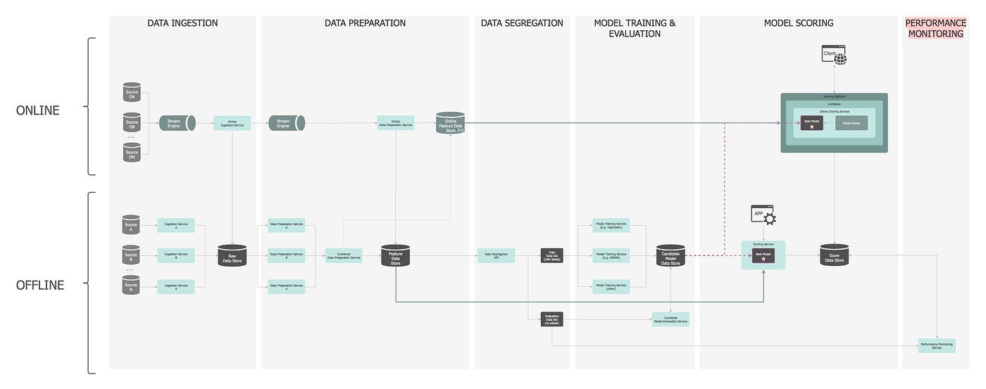
Any ML solution requires a well-defined performance monitoring solution. An example of information that we might want to see for model serving applications includes:
• model identifier,
• deployment date/time,
• number of times the model has been served,
• average/min/max model serving times,
• distribution of features used.
• predicted vs. actual/observed results.
This metadata is calculated during the model scoring and then used for monitoring.
This is another offline pipeline. The Performance Monitoring Service, is notified when a new prediction is served, executes the performance evaluation, persists the results and the relevant notifications are raised. The evaluation itself takes place by comparing the scores to the observed outcomes generated by the data pipeline (training set). The basic implementation for monitoring can follow different approaches with the most popular being logging analytics (Kibana, Grafana, Splunk etc).
To ensure built-in resilience of the ML system, a poor speed performance of the new model triggers the scores to be generated by the previous model. A "better wrong than late" philosophy is adopted: if a term in the model takes too long to be computed, the model is substituted by a previously deployed model, rather than blocking.
Additionally, the scores are joined to the observed outcomes when they become available — that means that continuous accuracy measurements of the model are generated, and along the same lines with speed performance, any sign of degradation can be dealt with by reverting to the previous model.
A chain of responsibility pattern can be used to chain the different versions together.
Model monitoring is a continuous process: a shift in prediction might result in restructuring the model design. Providing accurate predictions / recommendations continuously to drive the business forward is what defines the benefits of ML!
Cross Cutting Concerns
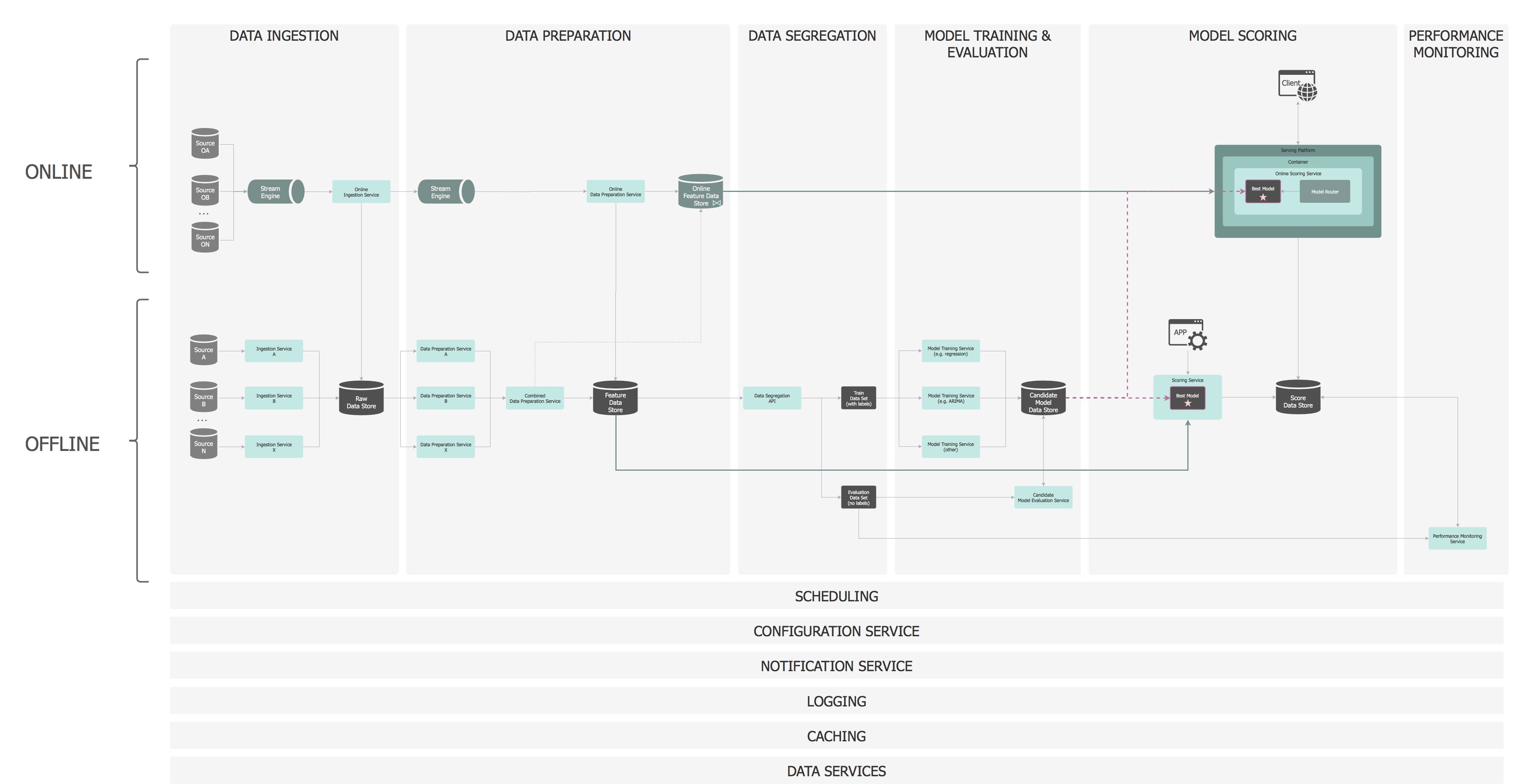
We cannot end this article by not referring to the cross cutting concerns. A ML application, like any other application, has some common functionality that spans across layers/pipelines. Even in an individual layer, such functionalities could be used across all classes/services, cutting through and crossing all the normal boundaries.
The cross cutting concerns are normally centralised in one place, which increases the application's modularity. They are often managed by other teams in the organisation or are off-the-shelf / thrid-party products. Dependency injection is the best way to inject these in the relevant places in the code.
The most important concerns to be addressed, in our use-case are:
• Notifications
• Scheduling
• Logging Framework (and Alert mechanism)
• Exception Management
• Configuration Service
• Data Service (to expose querying in a data store)
• Auditing
• Data Lineage
• Caching
• Instrumentation
And putting it all together
There you have it… A production ready ML system:
Footnote
Congratulations! You made it till the end! I do hope you enjoyed the ride into Software Engineering for Data Science!
Thanks for reading!
🙏🏻 💎 It has taken more than I originally anticipated to put this post together; having had to juggle things around — family/work demands/etc. Big shout out to my husband who was putting up with all these late nights! You are a gem!
I regularly write about Technology & Data on Medium — if you would like to read my future posts then please 'Follow' me !
Designing Machine Learning Pipelines Using Reinforcement Learning
Source: https://towardsdatascience.com/architecting-a-machine-learning-pipeline-a847f094d1c7
0 Response to "Designing Machine Learning Pipelines Using Reinforcement Learning"
Post a Comment